The mean, median and mode are 3 useful measures that tell us information about a data set.  The mean and the median tell us about the ‘central’ part of the data, and the mode tells us about the most commonly occurring value in the data.

However, a typical data set also has other characteristics.  For instance, look at these two simple data sets:

Data set 1	Data set 2
0, 5, 10, 15, 15, 20, 25, 30	12, 13, 14, 15, 15, 16, 17, 18

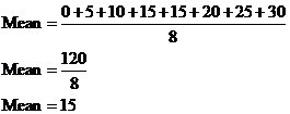
The mean of both data sets is 15 (check it if you don’t believe me).  The median of both sets is 15.  The mode of both sets is 15 as well.  But if we just look at the data sets ourselves, we can see that they are very different, even though they have the same mean, median and mode.  Data set 1 is a lot more spread out than data set 2.  To help describe how much the values in a data set are spread out, there are some measures of spread we can use.

Range

The range is a very easy measure of spread to understand – it’s the difference between the smallest value and the largest value.  For our sample data sets, the range can be calculated like this:

                                                    

As you can see, they have very different ranges. 

Quarters and quartiles

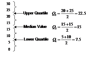
You can split the data up into quarters by arranging it in order of value, and then dividing it up into four equally sized groups.  For instance, the first data set could be divided up into quarters this way:

Quartiles are different to quarters.  Quartiles are the values between the quarters.  There are two commonly talked about quartiles, the upper quartile and the lower quartile.  The lower quartile is the value one quarter of the way up the values, and the upper quartile is the value three quarters of the way up the values.  The value one half of the way up the values is just the median, which we’ve looked at before.

Because we have 8 values, there is no value exactly one quarter of the way up the values.  So to work out the lower quartile, we need to take the average of the values just below a quarter of the way up (5) and just above a quarter of the way up (10).  This gives us a lower quartile value of 7.5.  The symbol for the lower quartile is often written as Q₁.

Same for the upper quartile – we have no value exactly three quarters of the way up, so we’re going to have to take an average.  The two values are 20 and 25, so the upper quartile has a value of 22.5.  The symbol for the upper quartile is often written Q₃.  What about Q₂ you may ask.  Well, Q₂ is the symbol for the median value.

Interquartile range

The interquartile range is the difference between the upper quartile and the lower quartile.  For our example, this is:

                                         

Deviations

The word deviate means to stray or to differ – in a mathematical sense the word ‘deviation’ describes how much the values in a data set differ from the ‘central’ value.

Mean deviation

The mean deviation is the average difference between the values in the data set and the mean of the entire data set.  So say we were finding the mean for data set 1.  We’d need to follow this procedure:

·         Find the mean of the entire data set

·         Find the difference between every value and the data set mean, as a positive number.

·         Add up all these differences and then divide by the number of values

                                

Once we’ve found the mean of the entire data set, we need to find all the differences.  Whether the value is larger or smaller than the mean, we need to give the difference as a positive number.   Think about it this way – we don’t care that much whether a value is above or below the mean, we just care how far away it is from the mean.  We can always have a positive number by picking the larger of the mean and the value, and subtracting the other number from it.  For instance, for the value ‘0’, the difference from the mean can be found like this:

                             

Last step is to add all these differences up and divide by the number of values, which is 8:

                          

So which is a better way to indicate how spread out data is?  Well, the range is quick to calculate, but the mean deviation is a more robust measure.  By robust, we mean that it is not too affected by one single very large or very small value.  For instance, take the following data set:

                                                        10, 11, 12, 243

The range for this data set is 233.  The mean deviation is 87.  The mean deviation is not so affected by the single large value, and hence is smaller than the range.  This is generally a good thing.