Sometimes you’re given a table of data and asked to determine whether an inverse relationship exists. What you can do is draw up a table and calculate the values of various products of the two variables. For instance, if we were given this data:
|
x |
1 |
2 |
4 |
8 |
|
y |
64 |
16 |
4 |
1 |
If there is a power 1 inverse relationship  , then the
product
, then the
product  will
be constant. If there is a power 2 inverse relationship
will
be constant. If there is a power 2 inverse relationship  , then the product
  will be
constant. Same goes for higher and higher powers. So here’s a table drawn up
with each of these products:
will be
constant. Same goes for higher and higher powers. So here’s a table drawn up
with each of these products:
|
x |
1 |
2 |
4 |
8 |
|
y |
64 |
16 |
4 |
1 |
|
|
64 |
32 |
16 |
8 |
|
|
64 |
64 |
64 |
64 |
The row doesn’t have constant values
along it, but the row does. This means that the
relationship is an inverse squared relationship, y is inversely proportional to
x2:

To work out the actual equation of the relationship, we need to work out what the ‘k’ constant is in the general form of the inverse squared relationship:

We can do this by substituting in the values from any pair of (x, y) values:
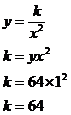
In this case I used the first pair of values, (x, y) = (1, 64). So k = 64. This means the exact inverse relationship for this table of data is:

More than two variables in a relationship – joint variation
The most well known formula in the field of electricity is this simple one:

It simply says that the (V)oltage in a circuit is equal to the current (I) in the circuit multiplied by the total (R)esistance of the circuit. Now, neither ‘V’, ‘I’ or ‘R’ are constants, they are all variables which can change their value. We would say that V varies directly as ‘I’ and directly as ‘R’.
We could of course rearrange this equation to make ‘R’ the subject for instance:

Now R also depends on two variables – ‘V’ and ‘I’. However, now we would say that R varies directly with ‘V’ and inversely with ‘I’ (since I is now on the denominator of a fraction).
Another common mathematical area where we have joint variation is anything to do with volumes. For instance, say we were designing a new rectangular swimming pool with a constant depth. In designing the pool there are 3 variables we can fiddle with – the width, length and height (depth) of the pool. The total volume of the pool is given by:

In this case, the volume of the pool varies directly with ‘w’, ‘l’ and ‘h’. Now say we wanted to fill the pool with ice instead of liquid water. We want to know how much the ice in the pool is going to weigh. Ice has a density of about 900 kg / m3. So we could rewrite the formula:

The ‘0.9’ in this case could be thought of as a constant ‘k’.
Most questions on joint variation will sound something like, “we’ll give you the values of all but one of the variables, work out the value of the one we don’t give you.”